FlowCell
Interactive motion and audiovisual experimentation — a dependency-free Canvas 2D environment for generative structures based on Fibonacci proportions.
Independent engineering & research project
Continuous Geometry. Deterministic Motion. Computational Engineering.
Exploring new approaches to interactive geometry, motion synthesis and computer-aided manufacturing.
O·C·E·A·N is an independent engineering and research project connecting computational geometry, motion control, CAD/CAM and digital animation. It is developed by Benjamin Thorsten Unger, a CNC/CAM practitioner with around two decades of machining experience. All research lines share one idea: describe geometry and motion continuously first, and discretise only when a machine, a renderer or a screen actually needs samples.
FlowSketcher, Infinity OvumPath, TSDE and TSDE TimeOS are separate projects with separate code bases and separate audiences. Choose the line you are interested in.
Browser-native geometry and CAM: tangent-continuous circular-arc chains (ArcFlow), biomorphic arc geometry (OvumPath) and native G2/G3 toolpaths for CNC machines.
Biomorphic geometry from circular arcs: an egg-shaped 2D contour, continued axially into two counter-wound strands, swept into 3D bodies with a Grasshopper sweep generator.
Velocity-driven motion synthesis for animation and camera motion: geometry, velocity and time are separated; frames are sampled from motion.
An operating system in the browser whose entire state is computed from an event log. Any earlier moment can be restored exactly, played back and taken as a starting point.
Interactive motion and audiovisual experimentation — a dependency-free Canvas 2D environment for generative structures based on Fibonacci proportions.
Sound from geometry: every track is a curve — Y shapes the pitch, X the timbre, with short and long hits on the beat below. Shaped with a stick, played with two buttons, recorded as a loop. Later as a standalone app and inside TSDE TimeOS.
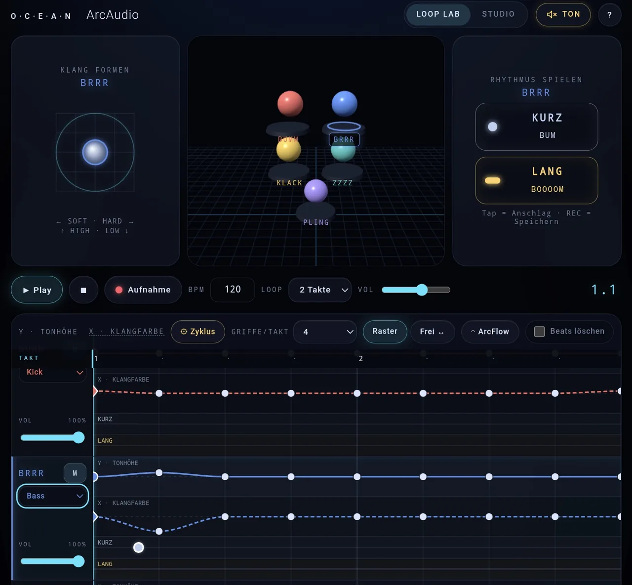
Feedback from people in audio is welcome. Write to me
FlowSketcher is a browser-native interactive 2D geometry environment with integrated CAM. The input is a movement of a finger, pen or mouse; the output is CNC-ready G-code. It runs on tablets, laptops and phones — no framework, no build system, no mandatory cloud service.
Pixel-based snap tolerance — endpoint, midpoint, centre, intersection, chain joints, construction lines, polar tracking, ortho — so snapping feels the same at every zoom level.
Every arc attached to an existing arc or line joins tangentially (C1) by construction. The user only chooses the side: G2 or G3. Lines, circles, Catmull-Rom splines, spline-to-arc conversion, fillets, offsets and SVG import complete the toolset.
Slots, arc slots, chain-following slots, rectangular and circular pockets, bores and pattern distribution along curves (FollowCurve) — all editable after creation without creating duplicates.
Vanilla JavaScript and Canvas. Command-pattern undo/redo with merged drag operations. No mandatory cloud service and no build environment.
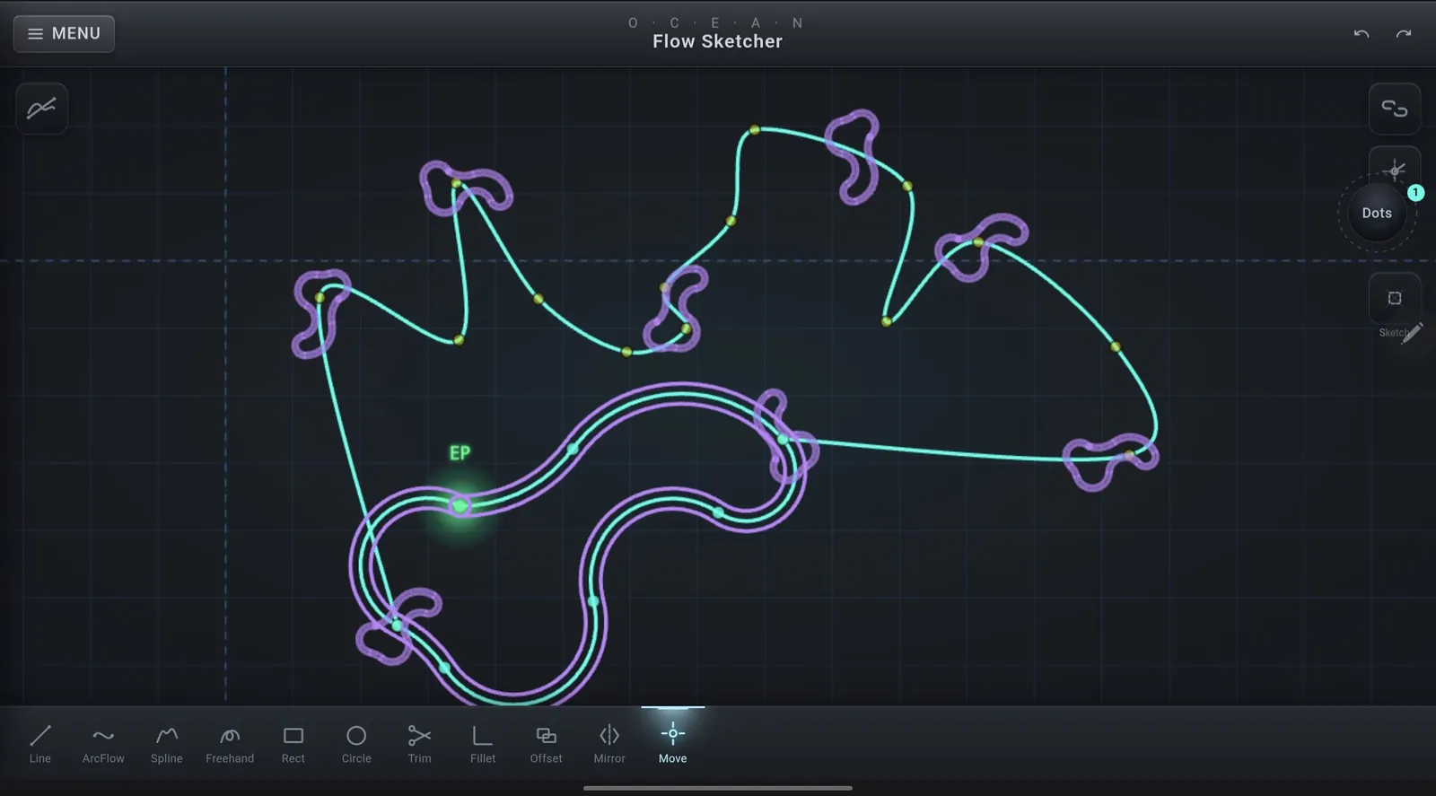
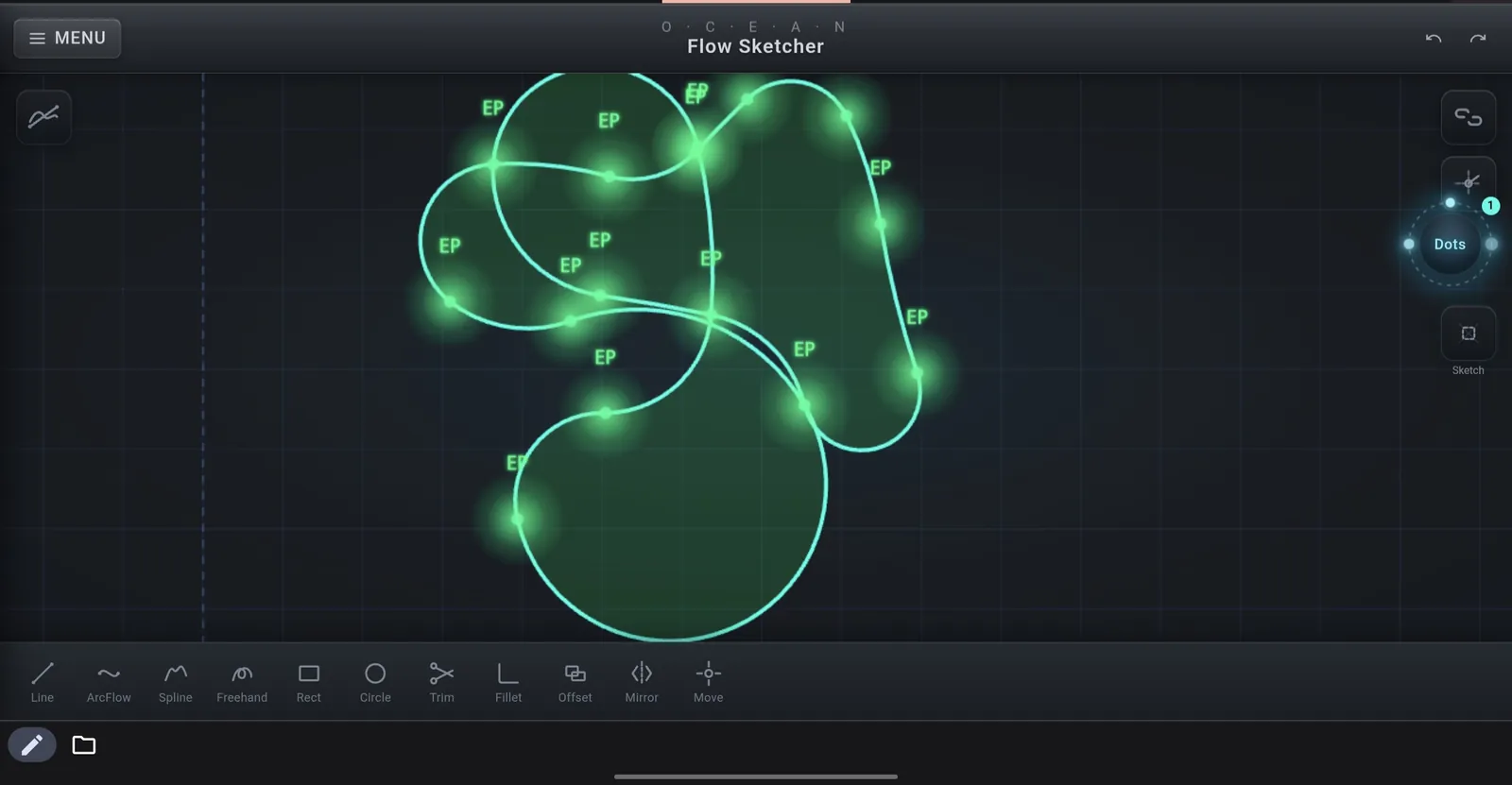
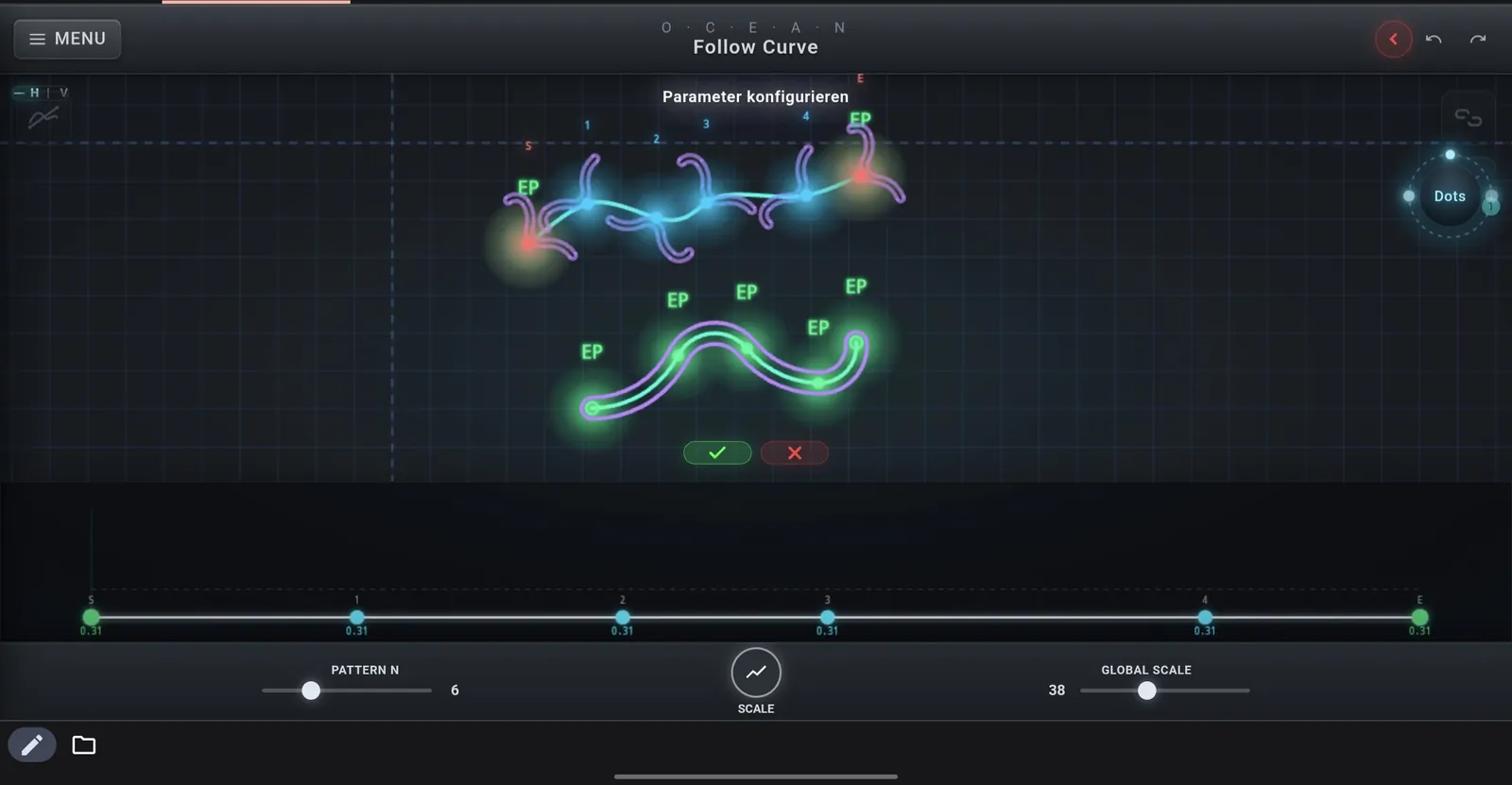
Not a complete commercial CAD platform, not a solid modeller, not a constraint solver and not 3D. It is a precision tool for people who know what G2 and G3 mean and who operate machines. The interface is minimal because every element is needed — not because simplicity is the goal.
ArcFlow constructs connected circular-arc chains with tangential continuity. Interactive manipulation updates dependent geometry through deterministic propagation.
Given a start point P, an incoming unit tangent T and an end point Q, there is exactly one circular arc (or, in the degenerate case, a straight line) that leaves P along T and ends in Q:
The end tangent of one arc becomes the start tangent of the next. Moving a point sends a propagation wave through all following segments; the chain behaves like a spring rod. Because only the direct predecessor supplies the tangent, propagation is deterministic and repeatable.
The objective is to preserve meaningful circular geometry instead of approximating everything with polylines — because circular arcs map directly to circular interpolation (G2/G3) on the control.
Closing a pure arc chain tangentially is checked live while dragging: green below 15° deviation, yellow from 15° to 35°, red when rotation directions are incompatible. Where the tangent does not fit, a closing blend (Catmull-Rom segment) bridges the gap with G1 continuity.
Import · SVG and splines become arcs
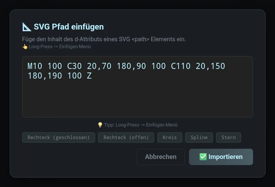
d attribute of any SVG path. The curve can then be turned into tangent arcs with Spline → Arc.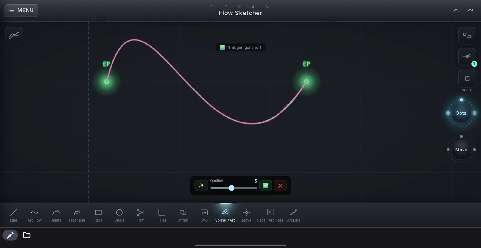
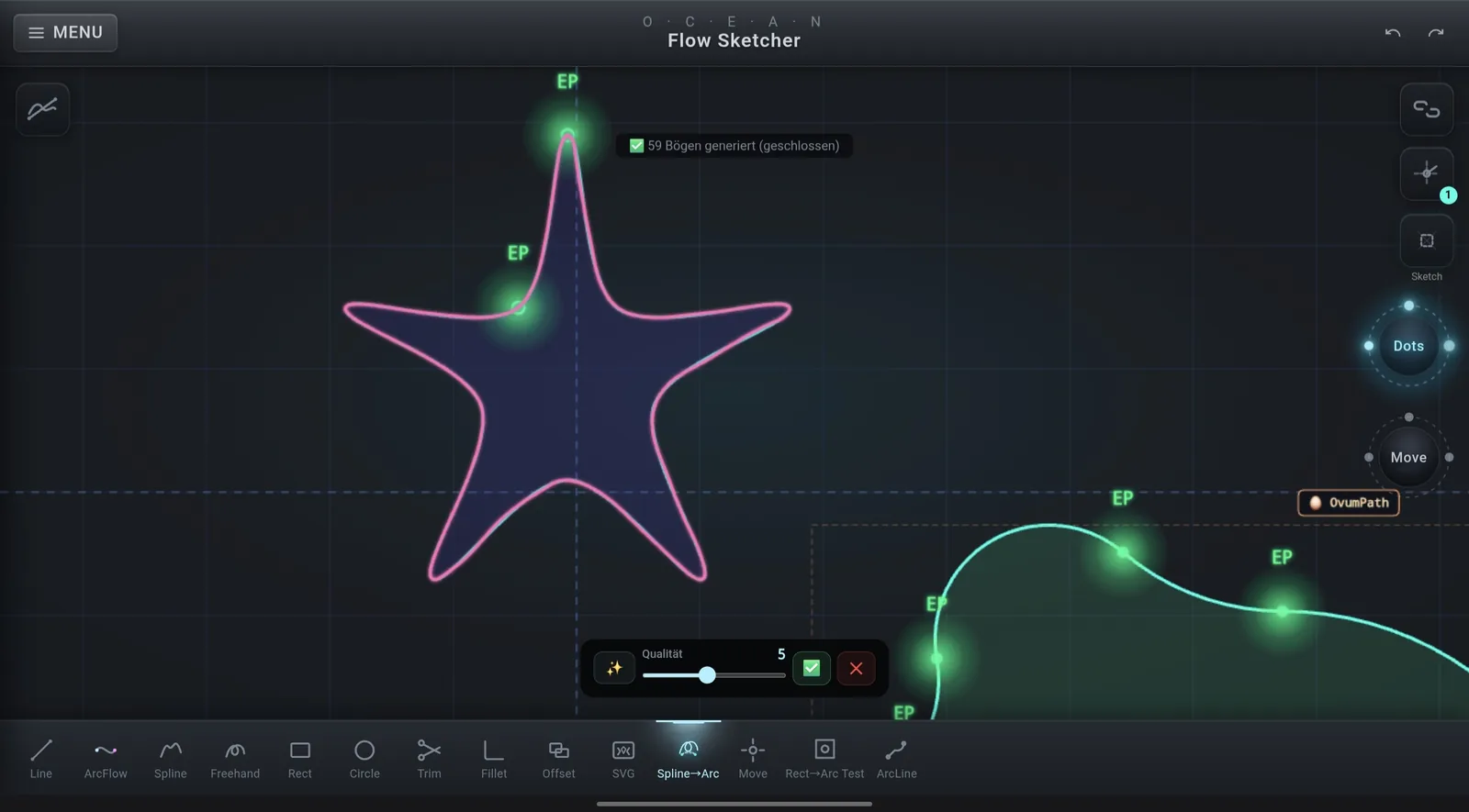
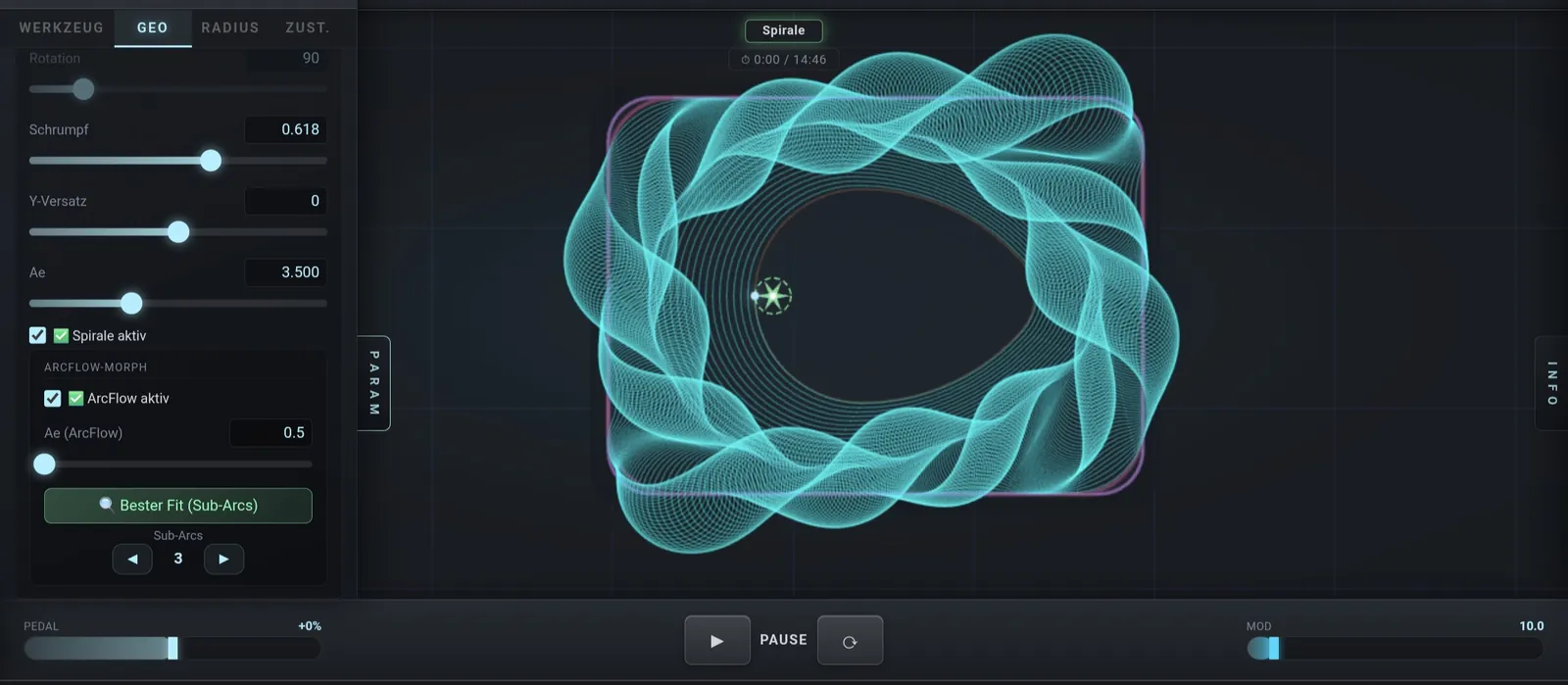
CR blocks in the NC program.Egg-shaped closed arc chain, morph spiral built from tangent arcs, live parameters and rubber-band control points.
Open the interactive ArcFlow demoArcFlow demo — link not yet configuredInside FlowSketcher, egg-shaped arc contours become machining geometry: offsets, morphs and spirals that stay exact circular arcs all the way to the NC program.
OvumPath is the only CAM tool that sits directly on an ArcFlow chain instead of a feature. It generates inward offset rings with collapse detection, then morphs from the inner shape over the last full ring back to the original contour, with an optional finishing pass. OvumCircPocket uses a radial correspondence — one ray from the egg centre through each vertex — so the morph does not twist, even for an eccentric egg.
The egg geometry itself — arc construction, axial continuation into the dual-strand egg helix, 3D sweeps and the utility-model publication — has its own research line.
Open Infinity OvumPath →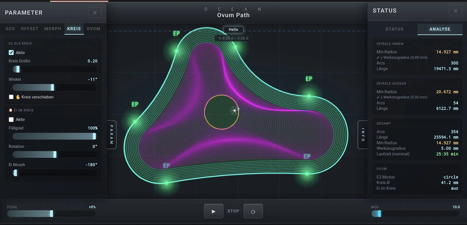
Each strategy picks a source, is configured in a panel, simulates live and is stored as a path on its source. All produce arc-based paths.
| Strategy | Principle |
|---|---|
| SpiralPocket | Helical plunge, spiral outwards, finishing pass, retract. Source: circular pocket or bore. |
| RectPocket | Morph from an inner shape (circle or egg) to the rectangular contour. |
| BossCam | Morph spiral from the picked feature to the outer stock contour (boss machining). |
| Circten | Circle and arc machining referenced to rectangular or circular stock. |
| OvumCircPocket | Circular pocket with egg morph and radial correspondence. |
| OvumPath | Free form on an ArcFlow chain: offset rings, collapse detection, morph back to the contour. |
ISO G-code (G1/G2/G3) and Heidenhain conversational (Klartext), optionally with mirrored X or swapped direction. Tool-edge paths with RL compensation — never centre paths; the control applies radius compensation. There is no approximation step between drawing and machine.
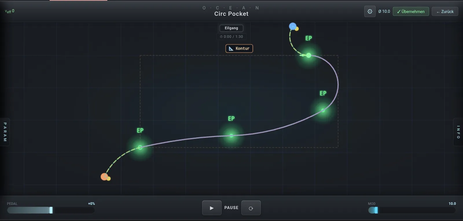
A toolpath is not only a shape. It is a sequence of blocks that a control has to read, plan and execute under physical limits. The geometric representation chosen in CAM affects every stage of that chain.
Tangent breaks force the axes to decelerate towards a stop at the corner. Tangent-continuous (C1) paths avoid these forced stops; curvature, however, still changes stepwise at arc-to-arc joints.
G2/G3 describe an arc exactly in one block (end point plus centre or radius). A polyline approximation needs many short G1 blocks and introduces chord error.
Spiral and morph strategies change the total path length and the share of cutting versus non-cutting moves. Length alone does not determine time; achievable feed matters as much.
Fewer, exact blocks mean smaller programs and less block-processing load. Where blocks are very short, block processing time can limit the effective feedrate.
On an arc of radius r at feed v, the normal acceleration is v²/r. With an acceleration limit a, the feed is bounded by v ≤ √(a·r) — small radii cost speed.
Look-ahead, jerk limits, servo tuning, contour tolerance settings and kinematics decide how a given path is actually executed. The same NC program can behave differently on different machines.
FlowCam keeps the arc as the primary entity from sketch to NC block. Before post-processing, the analysis panel shows for every path section the minimum radius against the cutter radius — so radii below the cutter radius are visible before the program reaches the machine.
Benefits of native arcs and tangent-continuous paths depend on the control, its parameters, the machine, the tool and the operation. Results from one setup must not be generalised to every machine or machining task. Measured comparisons belong in the benchmark laboratory.
Radius compensation only works if the control can offset the programmed path equidistantly. That needs a contour rather than a point sequence, tangent continuity, and inside radii no smaller than the tool radius.
Adaptive roughing cycles are usually computed as a centre path from an engagement calculation and output as G1 point sequences or approximated arcs. Neither is a finished contour the control could offset. To our knowledge there is no adaptive cycle on the market that outputs a compensatable finished contour.
ArcFlow reverses the order: the path is an arc chain from the start — every element a true circular arc, every joint tangent by construction. A morph spiral with 658 CR blocks ran completely under RL on an iTNC 530.
Control-side adaptive cycles exist as paid software options for newer controls (e.g. Heidenhain OCM); they work on the pocket and boss shapes the cycle can describe. ArcFlow addresses the CAM side: any arc contour becomes an adaptive path that leaves the CAM system as a compensatable contour — and also runs on older controls such as the iTNC 530.
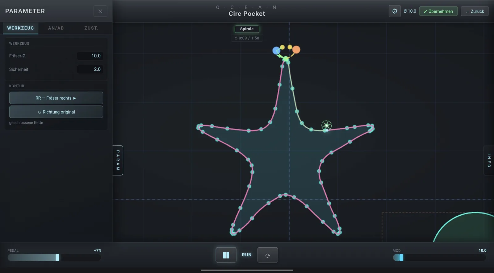
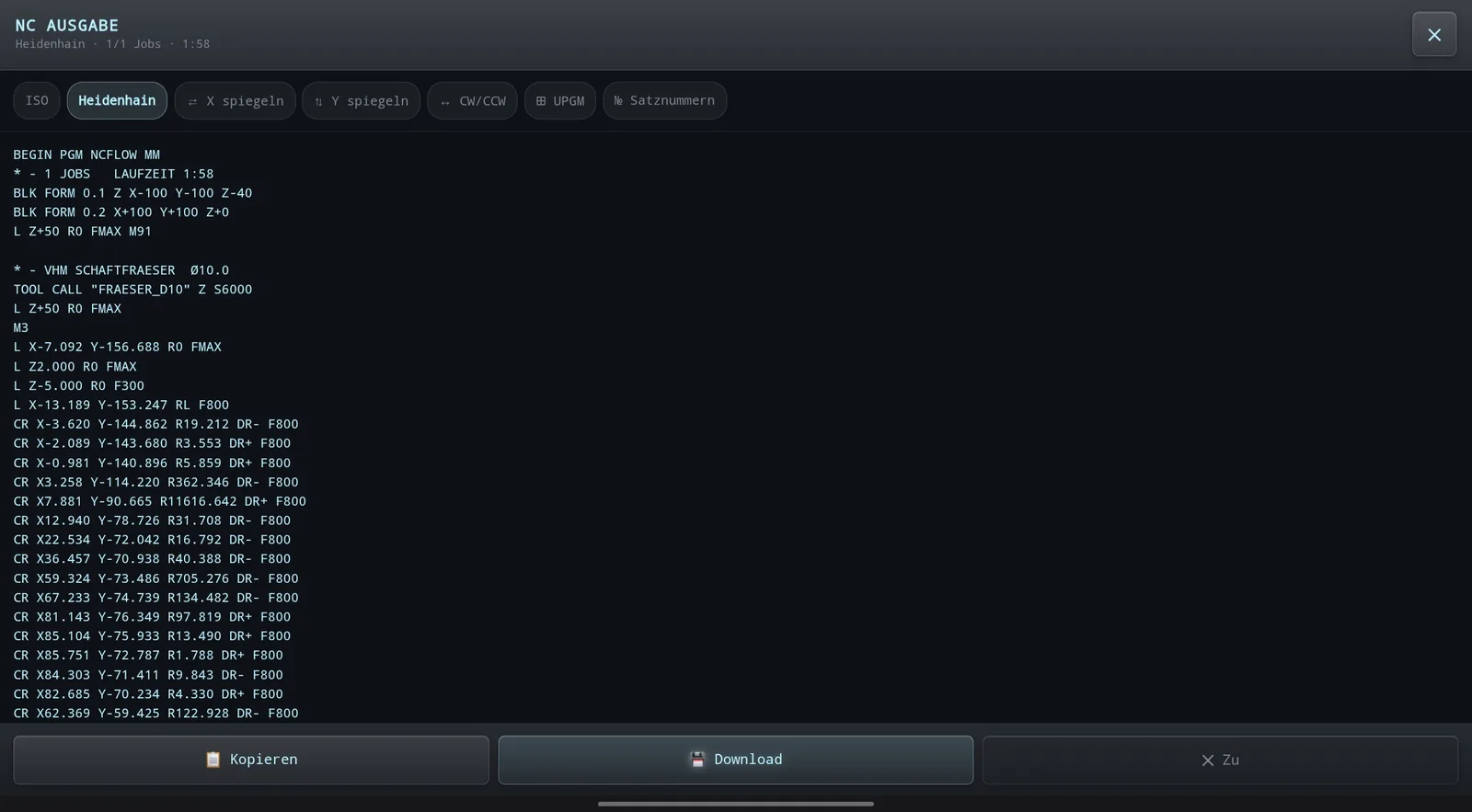
L … RL on the approach line, then only CR blocks with DR+/DR−. No G1 chain, no tolerance band.Claims about toolpaths should be tested on machines, under documented conditions, with data others can check. This laboratory separates what has been observed from what still has to be measured.
First comparison on a real machine against the established adaptive roughing strategy of a commercial CAM system (anonymised). Rectangular boss, same removal volume, one depth step, roughed. FlowCam is the reference; the values show the difference of the comparison strategy.
| Item | FlowCam | Comparison |
|---|---|---|
| Control | Heidenhain iTNC 530, same machine for both | |
| Run time | Reference | +20 s |
| Path length | Reference | +2 m |
| Advantage in ae and vf | — | yes |
| Extra finishing pass | yes | no |
| Radius compensation | RL over the whole path | centre path |
| CYCL 32 tolerance | no influence on time | up to 5 s difference |
FlowCam was shorter despite giving the comparison more step-over and feed, and despite running an additional finishing pass. Its run-time forecast matched the machine. A side finding — the control visibly paused at one corner because short sub-arc blocks fell below the block processing time of the iTNC 530 — led to a hybrid subdivision in BossCam.
Limitations: one run on one machine, not independently reproduced. Tolerance series (T1.0 / T0.5 / T0.05, two runs each, time from the control counter) still open. Material and tool are not documented here.
I cannot run further benchmarks myself. The next measurements therefore come from Close Beta testers: real parts on their machines, documented so that others can check them. Every result field stays empty until it has been measured.
Status: Close Beta · testers wanted
Principles: identical machine, tool, material and fixturing for every compared strategy; multiple runs; times read from the control; raw data and NC programs published.
| Parameter | Documented as | Result |
|---|---|---|
| Machine model & control | Manufacturer, model, control, software version, relevant parameters | pending |
| Workpiece geometry & material | Drawing / CAD file, material grade, stock dimensions, fixturing | pending |
| Cutting tool & manufacturer | Manufacturer, product code, holder, stick-out | pending |
| Tool geometry & cutting parameters | Diameter, flutes, corner radius; vc, fz, ap, ae | pending |
| CAM strategy & software versions | Strategy, settings, CAM / post-processor versions for each compared path | pending |
| NC programs | Complete programs as executed, published for download | pending |
| Actual machining time | Read from the control, several runs per strategy | pending |
| Toolpath length | Cutting and non-cutting length per program | pending |
| Surface quality | Roughness measurement method, instrument and positions | pending |
| Dimensional measurements | Measured features, instrument, temperature | pending |
| Recorded machine footage | Uncut recordings of each run | pending |
| GoPro video documentation | In-machine camera views, synchronised with run logs | pending |
| Reproducible test conditions | Full protocol so a third party can repeat the test | pending |
FlowSketcher and FlowCam are looking for machinists, programmers and shops who run real parts: one contour, one pocket or one boss is enough. Simulations I can run myself — what is missing is footage and data from real machines. A negative result is explicitly welcome; all reports are published with their conditions.
What a test report should contain
At every joint, adjacent segments share the same point and the same tangent direction (strictly, C1 refers to a continuous first derivative of the parameterisation; G1 to a continuous tangent direction). ArcFlow chains are tangent-continuous by construction. Their curvature is piecewise constant and changes stepwise at arc joints, so they are not curvature-continuous (G2/C2).
G2/G3 represent an arc exactly in a single block. Approximating it with straight G1 segments requires many blocks, introduces chord error and can let block-processing time limit the feedrate. Native arcs keep programs compact and preserve design intent such as radii and centres. The actual benefit depends on the control, its tolerance and smoothing settings, and the machine.
Curvature is κ = 1/r. Moving at speed v along a curve requires a normal acceleration of v²·κ, so an acceleration limit caps the speed at √(a_max / κ). Tangent breaks require stopping at the corner, and sudden curvature changes produce jerk.
Yes. G-code and Heidenhain conversational programs are text, and browser JavaScript can compute geometry and write that text locally without a server — FlowSketcher does exactly this. As with any CAM system, programs must be checked by simulation and by a qualified operator against the specific machine, control and post-processor settings before running.
Complete documentation of machine, control and parameters, tool and holder, material and fixturing, cutting data, CAM and post-processor versions; published NC programs; times read from the control over several runs; stated measurement methods for surface and dimensions; and identical conditions for every compared strategy, so a third party can repeat the test and obtain comparable data.
Organic forms, built from exact geometry: an egg-shaped contour made of tangent circular arcs, continued along an axis into two counter-wound strands, and swept into three-dimensional bodies.
Organic-looking contours can be constructed from circular arcs whose joins share tangent directions. Parameters that change radii, arc positions and transitions create families of egg-like or biomorphic shapes while preserving a circular-arc representation.
Infinity OvumPath explores this relationship between geometric construction, parametric shape generation and interactive morphing. A contour is both a visible form and geometry that can be offset, transformed or used as a machining boundary — the same arcs that appear in FlowSketcher's OvumPath CAM tool.
Tangency alone does not make curvature continuous: at each join the radius changes stepwise. That distinction matters as soon as a shape becomes a motion path or a toolpath.
The utility-model publication describes a guide curve generated by axial continuation of a single closed, egg-shaped two-dimensional contour. Iterative multiplication and axial displacement of this contour produce exactly two counter-wound helical strands that cross repeatedly along the longitudinal axis.
The publication further describes:
The mathematical derivation and generation variants are proprietary and not disclosed — neither in the publication nor on this page.
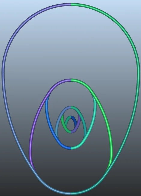
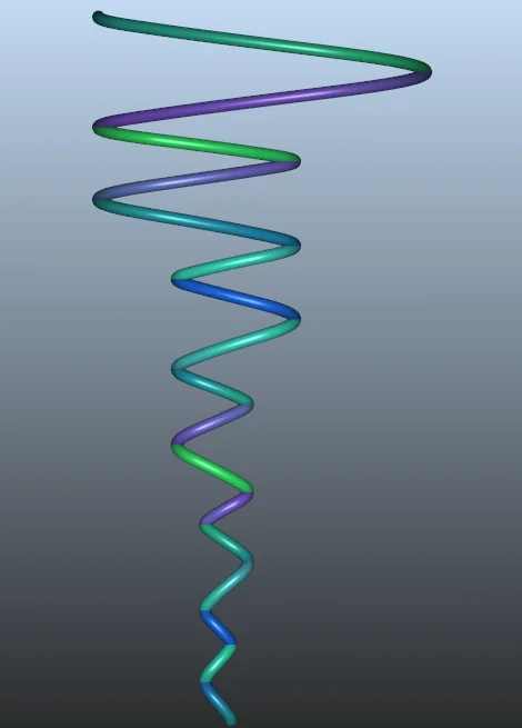

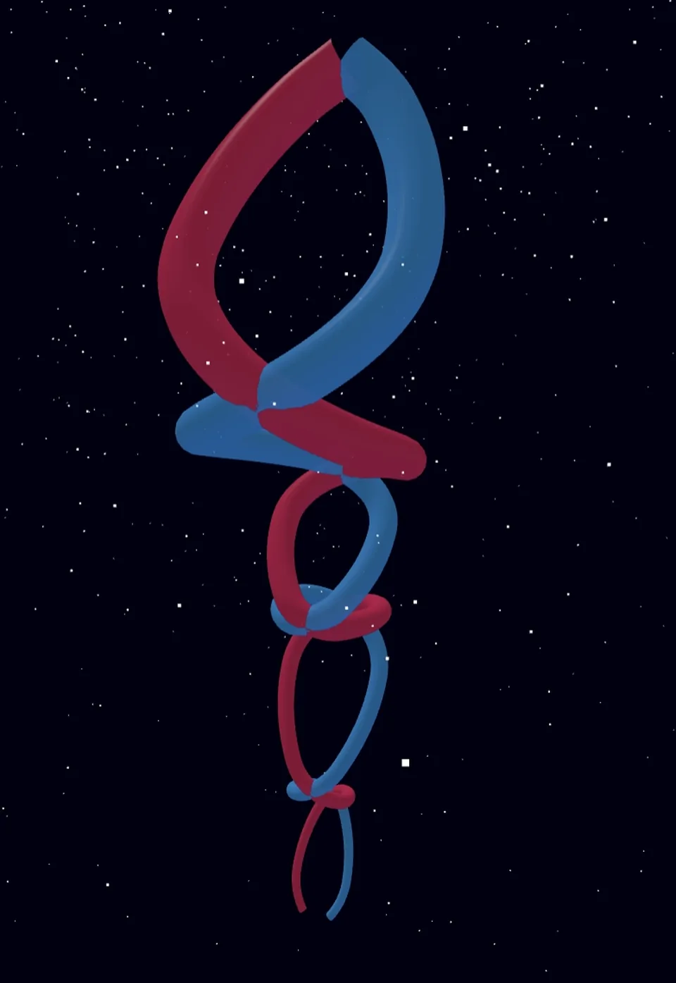
Light background: the egg-helix desktop software (V1.01, not released) — top view of six nested egg contours and side view of the resulting strand. Dark background: an internal viewer showing both strands as CCW and CW point clouds (CSV, 1,356 points each), drawn as tubes.
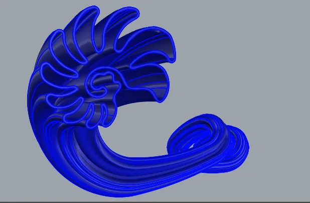
A Rhinoceros/Grasshopper plugin turns the guide curve into solid geometry: a cross-section is swept along both strands of the egg helix.
The clip shows rendered sweep results. Generation speed and scaling method are stated as described in the utility-model publication; no independent benchmark is published.
Text version provided by the German Patent and Trade Mark Office (DPMA), without drawings.
English summary for orientation; the German wording of the publication is authoritative. German utility models are registered without substantive examination of novelty and inventive step. This page makes no claim of worldwide novelty or uniqueness.
The publication names a broad set of potential application fields. They are listed here as named — without measured evidence, which has not been published for any of them.
Adaptive support structures for 3D printing, CAM milling strategies, load-bearing structures.
Targeted vortex formation in fluid media and flow optimisation are proposed; concrete implementations are reserved for future applications.
Sweeps with custom cross-sections, decorative objects, modular and educational construction systems.
Biotechnology and medicine (scaffolds, microfluidics), physics and astronomy (resonance models, simulations).
| Component | Status |
|---|---|
| 2D egg contour from tangent arcs | Implemented in FlowSketcher (OvumPath, OvumCircPocket) and the ArcFlow demo |
| Dual-strand egg helix | Documented registered utility model DE 20 2025 002 688 U1 |
| Grasshopper sweep generator | Documented results shown in the clip above |
| 3D viewer for the strand point clouds (CSV) | Internal not released |
| Egg-helix desktop software V1.01 (contours, helix, CSV spline export) | Internal not released |
| Open-source plugin for private use | Planned |
| CAM cycle for the egg helix | In development per the publication |
| Online ecosystem to configure and order 3D prints | Planned per the publication |
A guide curve obtained by continuing a closed, egg-shaped 2D contour along an axis. Repeating and displacing the contour produces two strands wound in opposite directions that cross repeatedly along the axis. Cross-sections swept along these strands produce three-dimensional bodies.
The 2D egg contour is built from tangent circular arcs — the same geometric principle as ArcFlow. In FlowSketcher the egg appears as a planar machining contour (OvumPath, OvumCircPocket). The helix and the sweep generator are a separate, three-dimensional line of work.
No. The utility model publishes the claimed structure and its description; the mathematical derivation, generation variants and the golden cross-section scaling remain proprietary. The four-arc egg on this page is a generic textbook construction used for illustration.
A sweep moves a 2D cross-section along a guide curve and generates the surface or solid it traces. Orientation and scaling of the cross-section along the path determine the final shape — which is where the sweep generator's scaling method comes in.
Traditional position-keyframe animation constructs motion by interpolating positions assigned to specific times. TSDE approaches the problem differently: it separates geometry, velocity and time.
A spatial path — a spline — defines where movement occurs. Its geometric unwinding (arc length) is computed per track.
A velocity function defines how movement progresses, in physical units (mm/s), driven by a per-track pedal between −100 % and +100 % of vmax.
Position is derived from accumulated distance along the path. Frames are generated only when the resulting motion is sampled for output.
We don't interpolate motion between frames.
We sample frames from motion.
As with audio, the mathematical description of the motion is independent of the output rate. The current TSDE engine advances its motion state on a deterministic fixed 240 Hz tick. Output frame rates such as 24, 96, 240 or 33.77 FPS are sampling settings applied to that motion — not the foundation of the motion model.
In a keyframe animation, timing is shaped by Bézier handles; the camera's speed is whatever the curve happens to produce. For fast camera moves this leaves large jumps between frames exactly where the motion matters most. The common workaround is to render at very high frame rates — often 240 FPS — and retime in post, discarding most of the rendered frames.
TSDE defines speed directly, in mm/s with realistic acceleration and deceleration — the way a motion-control rig or a vehicle moves. Frames are sampled at constant time steps from that motion, so a TSDE render folder reads like the output of a real camera. Slow motion and time-lapse are resampled from the same recording: you render the frames the target speed needs, not a surplus to throw away.
Output sampling rate (FPS)
Velocity profile (same path)
Display-rate playback
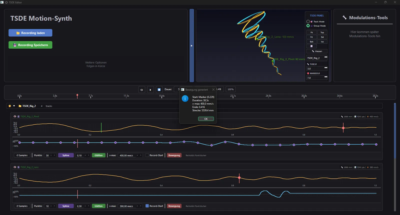
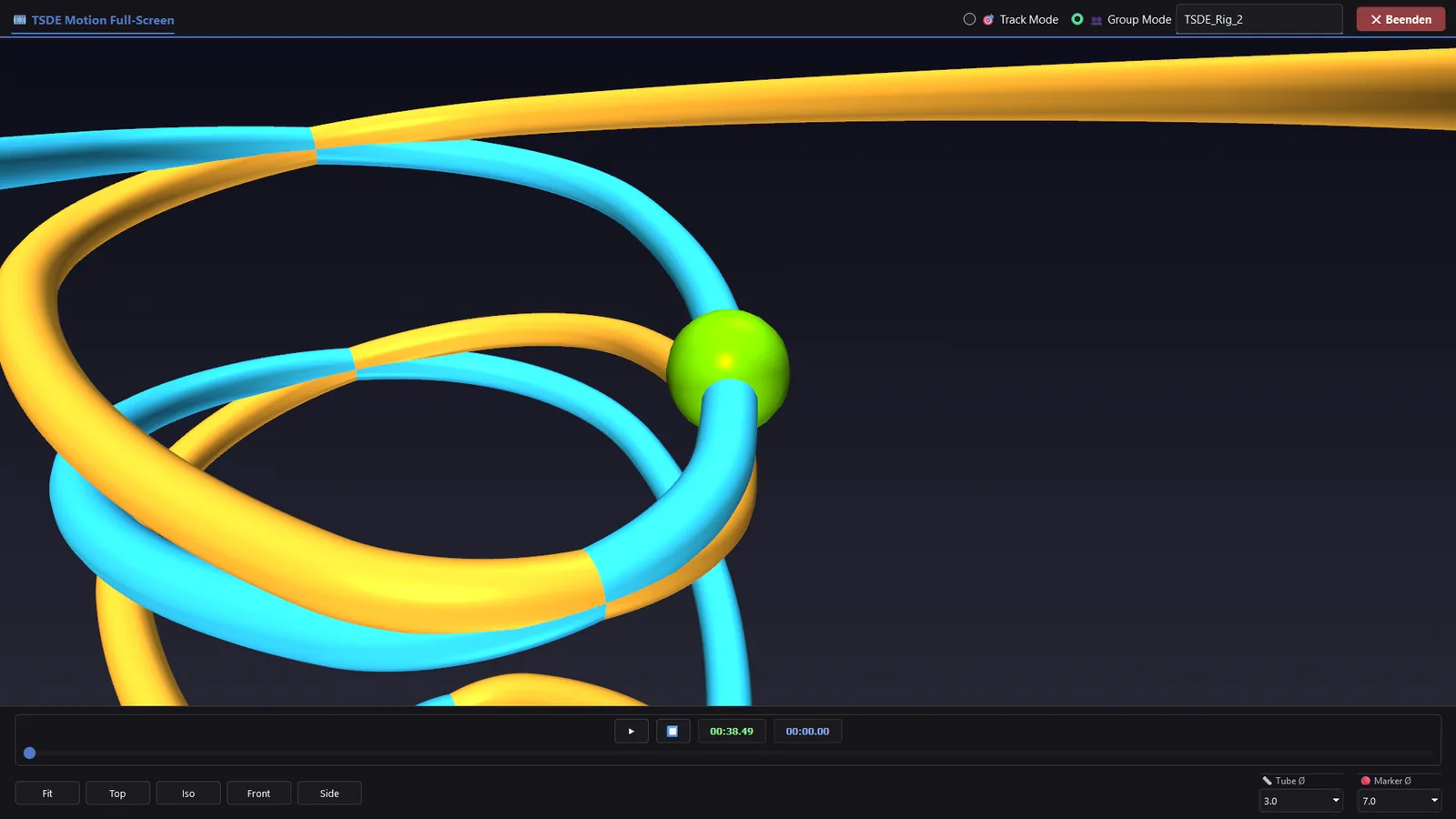
The toolchain follows the motion from its first recording to the final render — the same integration logic at every step.
Record
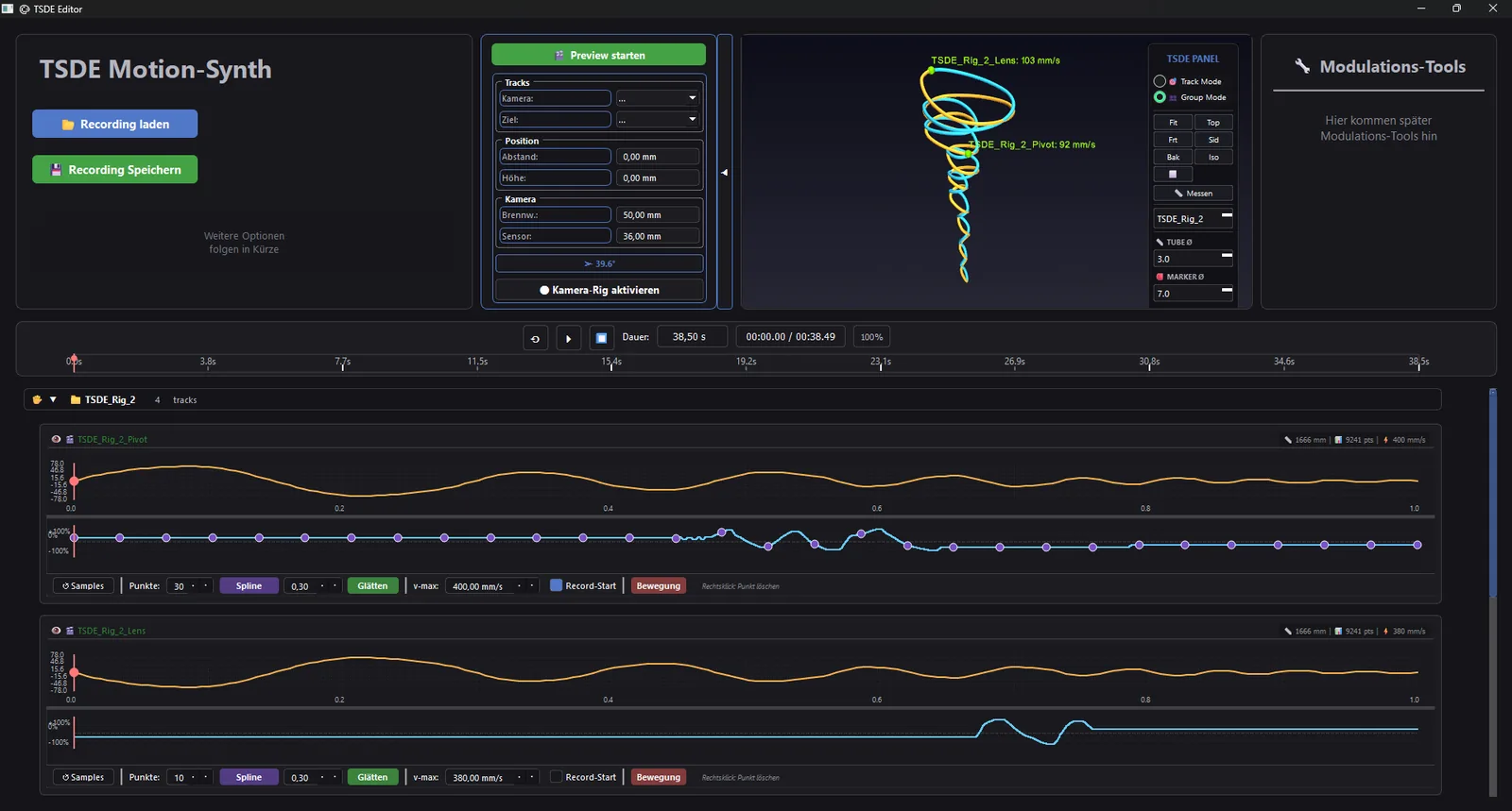
Edit & preview
With pedal value p(t) ∈ [−1, 1] per track:
Negative pedal values move backwards along the path; 0 % is standstill.
t byte-exactly.Modulation tools (noise, variation, pattern modulation), extended camera tools, multi-track camera rigs, live preview recording.
The Blender host connects the engine to an existing scene: paths come in from recordings or from existing animation, rigs are built automatically, and frames go out through Blender's renderer.
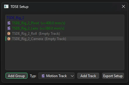
Builds complete camera rigs from curves: pivot, lens and roll empties, follow-path constraints set automatically, vmax configurable per track.
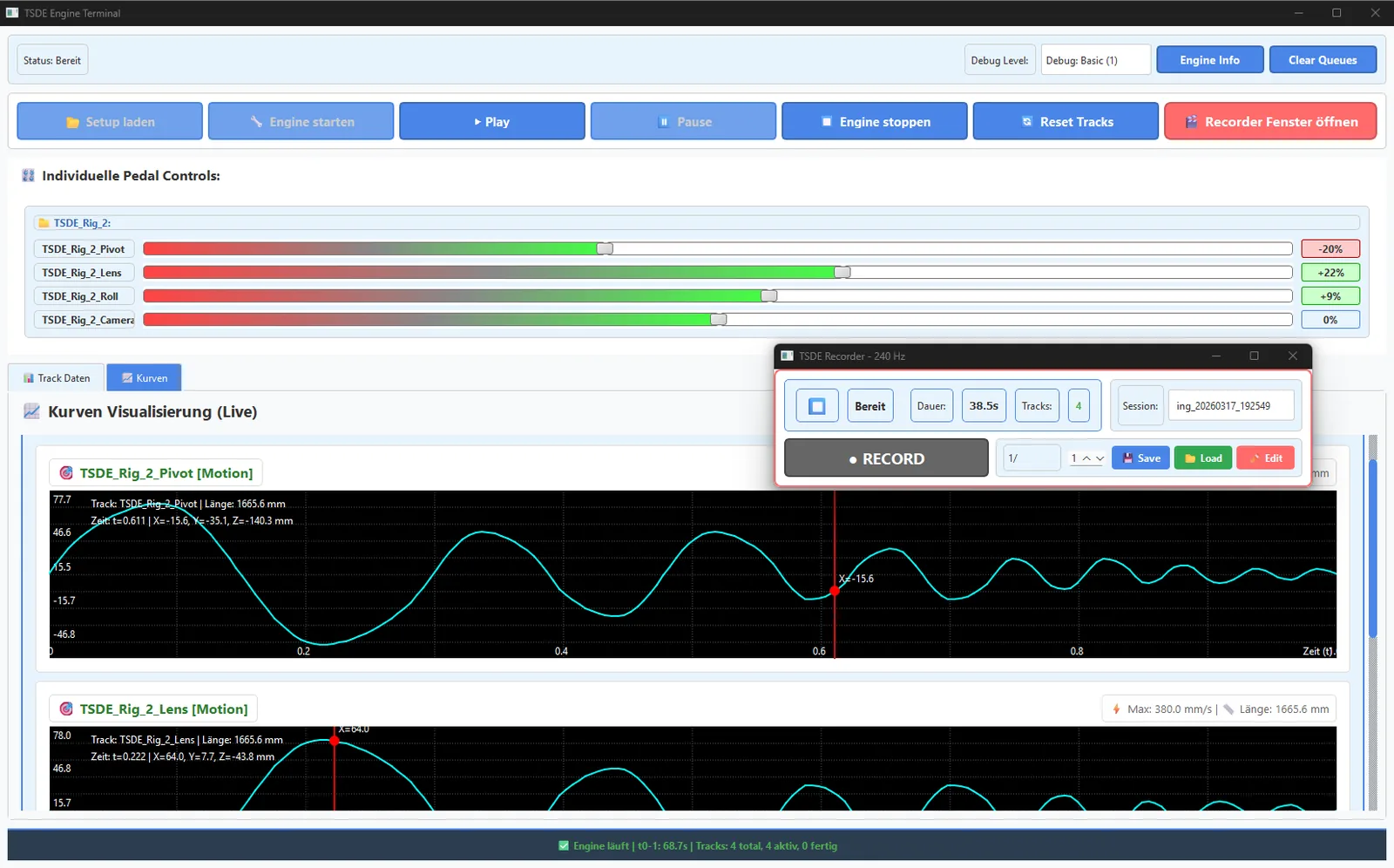
Start/stop, auto-export on changes, connection test (ping/pong), status monitoring. Play, pause and reset with manual pedal control and real-time feedback from the engine.
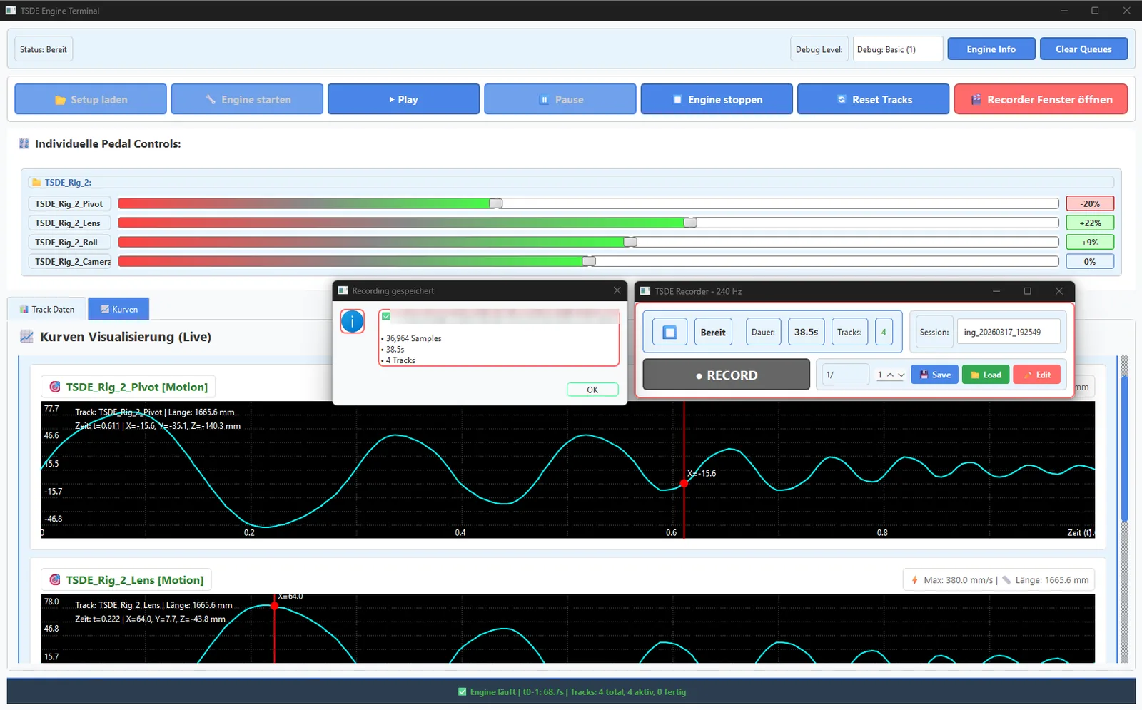
Runs in a separate process with deterministic storage, sample counter and status display.
Quaternion-based camera control with roll (no gimbal lock), multi-rig support, output manager for PNG, EXR and WebP, time-stretch rendering from 0.1× to 10×.
Sampling rates, keyframe decimation tolerance, control points per spline, export defaults and the time-stretch factor.
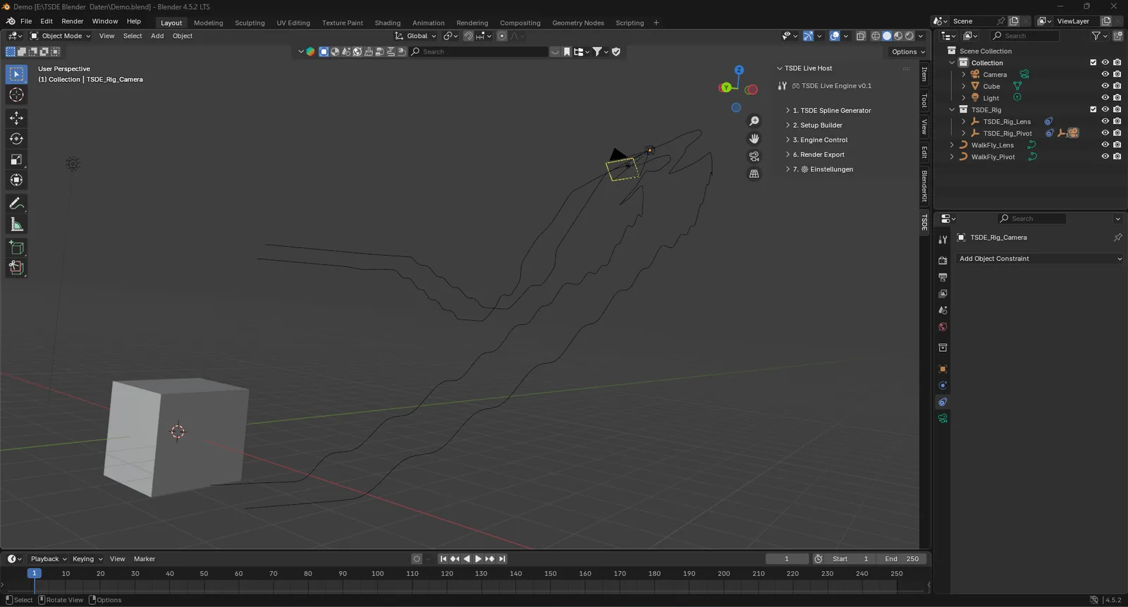
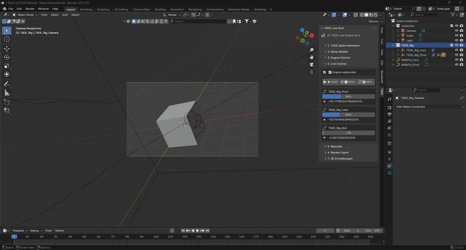
Blender host panels
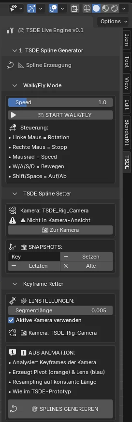
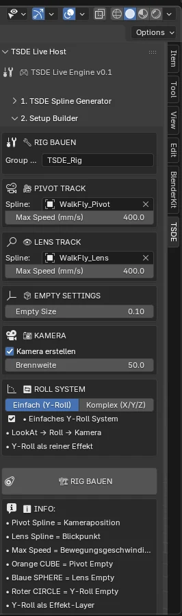
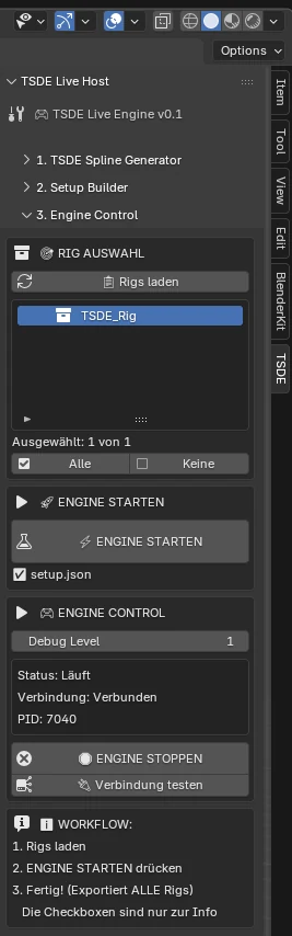
Spline Generator · Setup Builder · Engine Control.
Version 0.9 Beta. Because the time axis of a recording is kept unnormalised, one recording can be re-sampled into different outputs — including slow motion and time-lapse — without re-recording.
Motion is defined by a path and a velocity function over time. Position is not specified directly; it follows from integrating velocity to an accumulated distance s(t) and mapping that distance onto the path by arc length. In TSDE each track has its own velocity curve, driven by a pedal value scaled to the track's v_max in mm/s.
With keyframes, positions are assigned to specific times and intermediate positions come from interpolation curves; the timing of the movement emerges from those curves. With motion sampling, a continuous motion description exists first and output frames read it at chosen times — changing the frame rate changes the sampling density, not the motion. Keyframing remains the industry standard and offers direct pose control; the two approaches suit different tasks.
Timing can be edited without touching geometry, and geometry without disturbing timing. Velocity can be expressed in physical units, playback can be stretched (TSDE: 0.1× to 10×) from a single recording, and the path can be refined without changing how fast the motion progresses along it.
At speed v on a path of curvature κ, the lateral acceleration is v²·κ. Tight curves at high speed therefore read as abrupt; abrupt curvature changes read as jerks. Controlling velocity separately from the path lets the speed be reduced where the path bends, without editing the path itself.
TSDE TimeOS is an operating system in the browser in which nothing is ever overwritten. Every keystroke, every window, every song is an event on one shared timeline — and any earlier moment can be restored exactly: viewed, played back, or continued from.
There is exactly one source of truth: an append-only event log. Every event carries its tick k on a 120 Hz grid of absolute UTC time — the same tick on every device.
The state of every app is a pure function of the log up to time t. What is on screen is never stored; it is recomputed from the events — the present moment when live, any earlier one while scrubbing.
Each event is evaluated with the rule version that was in force at its tick. Shipped rules never change. That is why a recording made today will look exactly the same years from now.
We do not store states.
We store what happened.
The same idea as in line 3, one level up: there, motion is described continuously and only sampled into frames for output. In TimeOS, the history is the description — and the screen is merely its sample at time t.
The picture behind it is a cam drum: the motor is TSDE time, the cams are the tracks — pointer, touch, keyboard, windows, apps. Each cam emits time-stamped events.
Twelve seconds of history, 39 events. The screen on the left is folded anew from the log at every position of the slider — exactly how TimeOS works, only with millions of events.
Playhead (scrub)
Playback
The timeline sits at the bottom: sessions as light, pauses as a narrow seam. Drag to scrub, two fingers to zoom — from months down to a quarter of a second.
Last night's version of a text was better? Rewind, “record from here” — and carry on from exactly that state.
Replay shows more than content: windows, columns, the main menu, the tile layout and the app that was tapped are exactly where they were.
Flags with a note mark moments; the calendar shades each day by recorded time. One tap jumps right there.
System-wide, Ctrl+Z jumps back by one step — in every app, including embedded web apps. Nothing is swallowed silently.
One window manager for all devices: the log stores the logical place (“column 2 of 3”), never pixels. Each device draws it its own way.
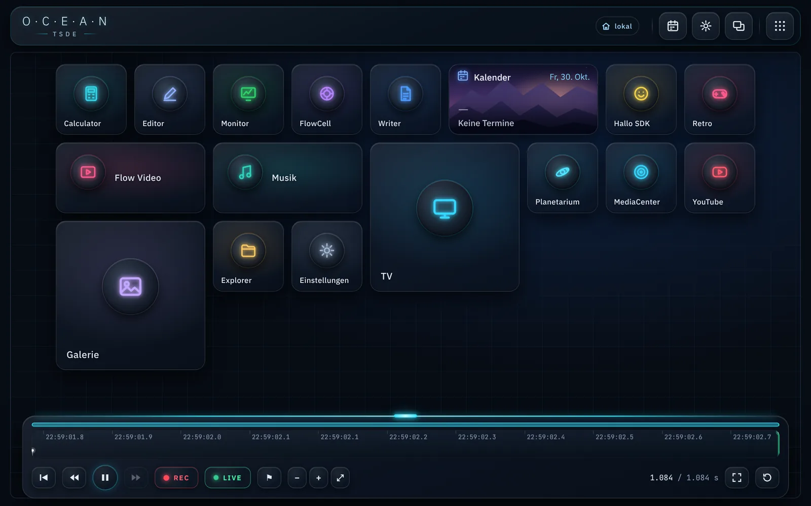
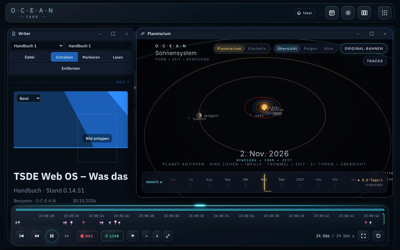
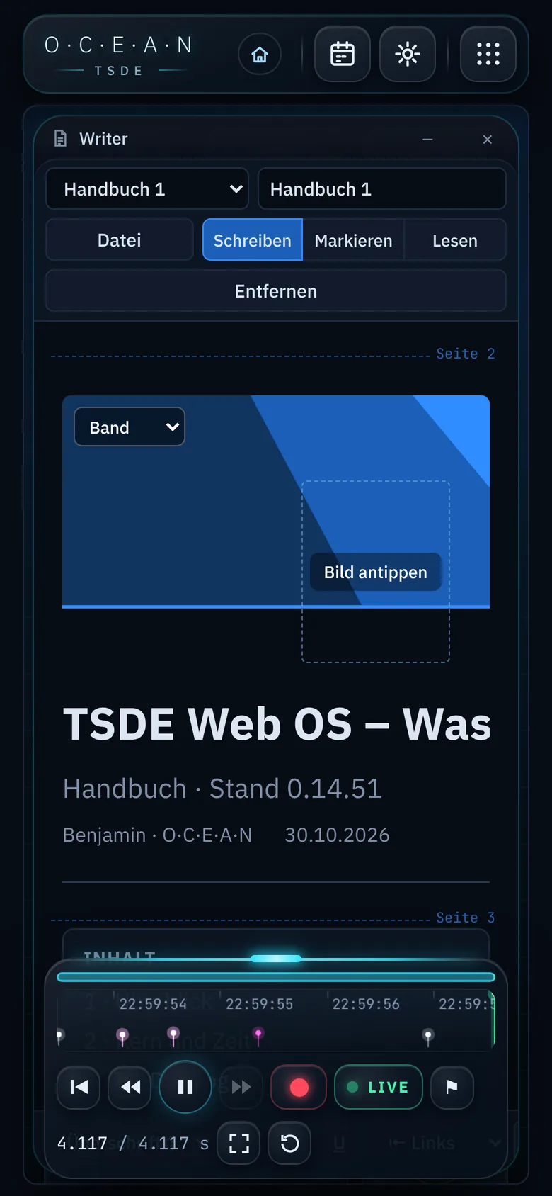
Every app follows the same rules — and gains abilities it could never have on its own.
| App | What time adds |
|---|---|
| Writer | Watch any text being written. Open and save DOCX, export PDF — own code, no third-party library. |
| Music | Web radio with a ring buffer: time-shifted listening, catch up to live, lift a song from the ring into the collection with ♥. |
| Flow Video | Playback as an anchor instead of a recording. From the ♥ favourites in Music it finds matching official clips: music TV from your own collection. |
| TV | The broadcaster's buffer is the ring — time-shifted viewing costs no storage; replay shows the picture of the time that was on air. |
| Retro | An N64 emulator on the timeline: inputs per frame in the log, replay recomputes bit-exactly. Rewind, take another path. |
| Planetarium | The solar system as a function of time, with the egg helix as orbit shape; the camera is computed in closed form so every replay is identical frame by frame. |
| FlowCell | A foreign web app under virtual time: clock, timers, randomness and frames come from the system — at every time mark the pixels match. |
A system that remembers everything must belong to no one else. So from day one:
TimeOS runs entirely on the device. Not a single request leaves it at start-up — even the fonts ship with it.
No sign-up, no analytics, no ads, no telemetry. The only things that go out are what you tap yourself: a radio station, a video.
Music and videos stay on the device, the NAS or your own cloud. If a file is missing, TimeOS tells you which device has it.
One history on every device: only the log, encrypted on the device, accessed with an anonymous twelve-word key. The server sees nothing but unreadable blocks.
Closed blocks are immutable and carry the state before them. Start-up therefore takes the same time however long the history is; old blocks load only when you jump there.
Every ten seconds the open tail is folded again; the check value must match the live state. Device tests on iPhone, Android phone and tablet; in private testing with family and friends.
gap is the time skipped between two moments (pauses, replay before “record from here”) — it does not count as playback.
apply is a pure function: no clock, no randomness, no DOM, no network.Installable without a store with offline storage, sync without an account, branches instead of deletion when re-recording, an app shell for Android, a kiosk mode for Raspberry Pi and machine control.
An operating system in the browser by Benjamin Thorsten Unger (O·C·E·A·N) in which the entire state — windows, input, documents, media, games — is computed from a single event log. The timeline is the central control: any earlier moment can be restored exactly, played back, or taken as a new starting point.
No. Only events are stored — a keystroke, a window in place 2, playback from second 41. The picture is recomputed every time by folding. That keeps the history small: a block of 4096 events compresses to roughly a twelfth.
Undo and version control work per program or per file. Event sourcing is the well-known pattern underneath. TimeOS puts the whole system on one shared 120 Hz timeline — window manager, input, media playback, emulator and embedded web apps — and makes time itself the interface: you scrub through your day like through a video.
Through rule versions. The log states which rules applied; each event is evaluated with the version active at its tick. A shipped version is never changed — new behaviour is always a new version.
It enters the log as a result, not as a picture: which station, which title, which position. Radio can be recorded into a ring on request; TV uses the broadcaster's own buffer. Whatever can no longer be loaded later is marked “not reconstructable” in replay.
Not publicly yet. TimeOS is in private testing; a public, installable version is the next step. The principle stays: offline, no account, the data belongs to the user.